8. Demonstration

The motivation for this project was a need for paraglider flight dynamics models for commercial paraglider wings. The goal of this project was to build those system models by creating parametric component models that augment the limited available specifications with assumptions of the unknown structure. This chapter demonstrates one possible workflow to estimate the parameters of those component models by combining publicly available technical specifications and photographs with knowledge of typical paraglider wing design.

The paraglider wing used in this example is a Niviuk Hook 3. With forgiving flight characteristics targeting advanced beginners, this wing is not intended for acrobatics, so the limitations of the aerodynamics method are not an issue when simulating the majority of flights produced by this wing.

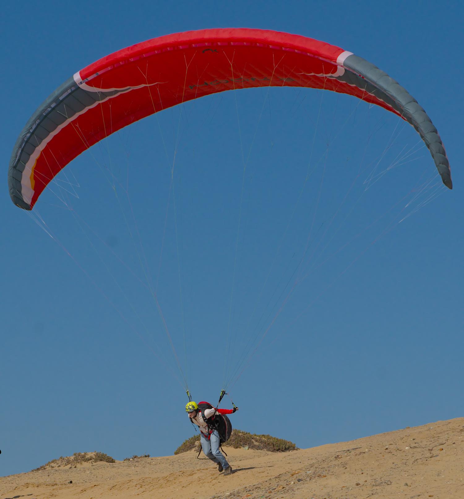
Fig. 8.1 Front-view of an inflated Niviuk Hook 3

Wing data for a commercial wing is typically limited to four sources:

1. Technical specifications and user manuals

2. Flight test data from certifications and reviews

3. Pictures and videos

4. Physical measurements

For this chapter, only the first three will be utilized. Although physical measurements are ideal, they are frequently difficult to obtain (especially for older wings). Instead, this demonstration is focused on showing that it is feasible to create an approximate wing model even if physical measurements are unavailable.

8.1. Technical specifications

The following sections demonstrate how to estimate the parameters for a size 23 version of the wing. The same process is used (but not shown) to create models of the size 25 and 27 wings to validate the modeling choices and implementation.

The process begins with the primary technical data from the official technical specifications manual:

Table 8.1 Wing data

Property [unit]	Size 23	Size 25	Size 27
Flat area [m2]	23	25	27
Flat span [m]	11.15	11.62	12.08
Flat aspect ratio	5.40	5.40	5.40
Projected area [m2]	19.55	21.25	22.95
Projected span [m]	8.84	9.22	9.58
Projected aspect ratio	4.00	4.00	4.00
Root chord [m]	2.58	2.69	2.8
Tip chord [m]	0.52	0.54	0.56
Standard mean chord [m]	2.06	2.14	2.23
Number of cells	52	52	52
Total line length [m]	218	227	236
Central line length [m]	6.8	7.09	7.36
Accelerator line length [m]	0.15	0.15	0.15
Solid mass [kg]	4.9	5.3	5.5
In-flight weight range [kg]	65-85	80-100	95-115

Recall that a “paraglider wing” includes both the canopy and the suspension lines, so the technical data describes both components. It also includes the weight range that the wing can safely carry while retaining control authority, which will be used to define a suitable payload.

8.2. Canopy

The first component model of the paraglider system is for the canopy. The canopy model combines an (idealized) Foil geometry model with physical details to estimate the aerodynamics and inertial properties of the canopy. For the canopy model parameters, it’s easiest to think of them in two groups:

1. Parameters for the design curves that define the variables (3.15) of the foil geometry model.

2. Parameters for the physical details (5.10)

8.2.1. Foil geometry

Layout

The first part of specifying a foil geometry is to layout the scale, position, and orientation of its sections.

For a parafoil, it’s easiest to start by describing the geometry of the flattened (uninflated) canopy before dealing with the arc. This approach is made much easier by the choice of the Simplified model to define the section index as the normalized distance along the $yz$-curve. When a parafoil is flattened the section index corresponds to the normalized distance along each semispan, which allows the $x$-positions and chord lengths to be measured directly without regard for the arc.

First, consider the chord length distribution $c(s)$. The technical specifications only list the root, tip, and mean chord lengths, so more information is required. Thankfully, for parafoils a reasonable guess is that the wing uses a truncated elliptical distribution. (Paragliding wings commonly use truncated elliptic functions because they encourage elliptical lift distributions, thus reducing induced drag.) Such a truncated elliptical distribution can be easily parametrized by the wing root and wing tip section chord lengths, as shown by the Elliptical chord design curve. The technical specs list these two parameters as $c_{\text{root}}=2.58$ and $c_{\text{tip}}=0.52$, respectively. Using those values produces a standard mean chord length of $2.06$, which exactly matches the value listed in the manufacturers specs, so the assumption was justified. An additional check is to compare the area of the flattened chord surface projected onto the $xy$-plane; for these values the truncated elliptical produces a flattened area of $22.986$ compared to the true specification of $23.0$, which further confirms the design. (The small discrepancy may be explained by differences in measuring methodology or by the current absence of any geometry twist, but in practice the effect is negligible.)

Next is the fore-aft positioning of the sections, which are controlled by the $r_x(s)$ and $x(s)$ design curves. Although traditional wing geometry models would effectively choose $r_x(s)=0$ and measure the $x$-offsets of each section’s leading edge, that choice often produces an unnecessarily complicated $x(s)$ function. Instead, paragliders can often be described with constant $r_x(s)$ and $x(s)=0$. As with the chord lengths, the value of $r_x(s)$ is easiest to estimate from the flattened wing; in fact, flattened drawings are commonly available in technical manuals, making them especially convenient. (Admittedly, such drawings do not always maintain the true aspect ratio, and so should be used with caution.) For this wing, a small amount of trial and error using a top-down view from the wing user manual suggests a constant $r_x(s)=0.7$ gives a strong agreement with the drawing in the manual, as seen in Fig. 8.2.

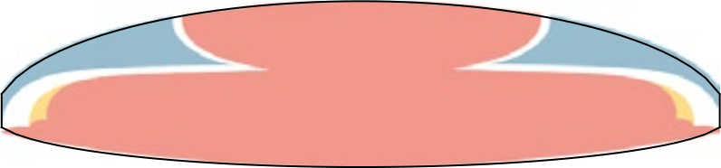
Fig. 8.2 Top-down outline of flattened canopy

The black outline is the boundary of the model’s flattened chord surface. The colored background is taken from the user manual for the wing.

With the flattened chord surface completed, the next step is to define the arc (position in the $yz$-plane) to bend the flattened surface into its characteristic shape. Photos of the wing suggest that an elliptical arc segment is likely. The exact value of the arc reference points $r_{yz}(s)$ has a minimal impact for typical parafoils (which have relatively small geometric twist), but a reasonable guess is to use the quarter-chord position $r_{yz}(s)=0.25$. For the arc positions $yz(s)$, an Elliptical arc can be defined using three parameters: two for the normalized shape (${\mathrm{\Gamma }}_{\text{tip}}$ and ${\varphi }_{\text{tip}}$) and one for the scale ($b_{\text{flat}}$). There are several ways to estimate the elliptical arc parameters of the physical wing, such as the width to height ratios, or visual estimation of the arc angle, but since the specs included both the flattened and projected spans, the simplest method is to guess a value for ${\varphi }_{\text{tip}}$ and increase ${\mathrm{\Gamma }}_{\text{tip}}$ until the projected span matches the expected value. Starting with an initial guess of ${\varphi }_{\text{tip}}=75$, a few iterations shows good agreement with ${\mathrm{\Gamma }}_{\text{tip}}=32$. Checking the fit shows a projected span of $b=8.845$ (versus the true value of $b=8.840$) and a projected area of $S=19.405$ (versus the true value of $S=19.550$). As with the flattened values, the small discrepancy may be explained by differences in measurement methodology, and likely isn’t worth optimizing further.

After the relatively straightforward process of positioning the sections is the more difficult task of estimating their orientation. In the simplified model, section roll $\varphi (s)$ is defined by the curvature of the $yz$-curve and the section yaw $\gamma (s)$ is defined as zero, but the section pitch $\theta (s)$ (or geometric torsion) can be difficult to determine (even with a physical wing in hand). Relying on the fact that parafoils commonly benefit from a small amount of increasing geometric torsion towards the wing tips (or washin), a conservative guess of 4° at the wingtip should be reasonably accurate [32]. For lack of better information, this demonstration chose a piecewise linear model that grows 0–4° degrees over the range $0.05\le |s|\le 1$.

Profiles

Having finished defining the section layout (scale, position, and orientation), each section must be assigned an airfoil [37]. The most accurate way to determine the section profiles would be to cut open the wing and trace the outline of the internal ribs, but in this case that’s not an option. Another option would be to search an airfoil database, but the simplest approach is to use a choice from literature. When using literature, it’s important to keep in mind that although papers discussing “parafoils” and “ram-air parachutes” have much in common with paraglider canopies, those papers are typically analyzing large canopies designed for heavy payloads.

From the ram-air category, [29] observes that many “older designs” use a Clark-Y airfoil with 18% thickness; it also mentions that “newer gliders” have been design with “low-speed sections”, such as the LS(1)-0417 (for example, see [45]). For literature targeting paragliders specifically, one option is the NACA 23015: a classic, general purpose airfoil used in the wind tunnel model [19]. Another paraglider-specific option is the “Ascender”: an 18% thickness airfoil developed for an open-design paraglider [32]; for an example of literature using that airfoil, see [46].

The criteria for selecting an airfoil is beyond the scope of this demonstration, but a key observation is the tendency for paragliders to use unusually thick airfoils. The reason for this is that thick airfoils tend to have more gentle stall characteristics, since their low-curvature leading edges encourage flow attachment as the angle of attack increases. Higher performance wings may select thinner airfoils to reduce drag, because the Hook 3 is a beginner-friendly wing this model uses a NACA 24018; it’s similar to the 23015 used by the wind tunnel model but with 18% thickness. (For the curious reader, using the Ascender airfoil barely changes the equilibrium conditions for the wing; small changes to the equilibrium pitch angles and a small increase in the range of airspeeds, but otherwise the change had a surprisingly small effect.)

After choosing an airfoil, the next step is to modify it support the brake inputs. The unmodified airfoil defines the section profiles when no brakes are applied, but a paraglider must deform those profiles in order to turn and slow down. This poses a significant difficulty with modeling a paraglider, since the deformation is a complex process. Unlike wings made from rigid materials with fixed-hinge flaps, the brakes produce a continuous deformation along variable-length sections of the profile. Instead of dealing with that complexity, this project uses a strategy to simply guess the deflected geometry.

To begin, observe that the trailing edge of a braking paraglider typically exhibits a transition region followed by a gentle curve. In the interest of practicality, model the transition and trailing regions as circular arc segments. (This modeling choice is made with no theoretical justification beyond the recognition that spherical shapes tend to appear as the energy-minimizing state of a flexible surface under tension.) Because this is not a theoretically well-justified model the algorithm will not be covered in detail, but this “two-circle model” can be used to generate a set of deflected airfoils.

Fig. 8.3 Two-circle model to generate an airfoil with a smoothly-deflecting trailing edge.

For the upper surface, first choose a point (a) at some distance from the trailing edge (c) and attach a circle C2 tangent to the airfoil at a and replace the transition region of the airfoil with an arc from a to b; then, place a second, larger, circle C1 tangent at b and draw another arc for the remaining length of the upper curve. For the lower surface, choose a point d some distance roughly equal to the modified length of the upper surface and use a Bézier curve to draw a deflected lower surface between d, the new trailing edge c, and the point where the deformed upper surface curve crosses the original (undeformed) lower surface curve. The radius of the smaller circle C2 controls the sharpness of the transition, and the radius of the larger circle C1 controls the maximum steepness at the trailing edge. This procedure maintains the length of the upper surface, but neglects the wrinkling that normally occurs along the lower surface.

Using this procedure with the NACA 24018 as the baseline produces a set of reasonable-looking curves:

Fig. 8.4 Set of NACA 24018 airfoils with trailing edge deflections.

At this point the reader should be highly skeptical of this airfoil set. The choice of airfoil, and how the airfoil deforms in response to trailing edge deflections, is full of assumptions. Nevertheless, these results will be used for the remainder of this chapter as a means to demonstrate the working of the model. As a result, an important thing to keep in mind when interpreting the results of these choices is that choosing such a large radius for C2 is wildly optimistic, but was chosen anyway to reduce the curvature of the transition region. For small brake inputs the transition curvature is negligible, but becomes progressively sharper as deflection increases. High curvature can be a problem for some theoretical models used to estimate the section coefficients (including the viscous/inviscid coupling method in XFOIL [47]), since the high curvature inhibits the method from converging on a solution when viscosity is taken into account. Softening the curvature allows the estimate to converge, but at the cost of hiding convergence failures that typically suggest flow separation. As a result, this profile set is likely to overestimate lift and underestimate drag.

8.2.2. Physical details

In addition to a foil geometry, a canopy model requires details of physical attributes such as surface material densities and air intake extents in order to calculate inertial properties and viscous drag corrections.

Surface materials

In this case, the surface material densities can be read directly from the materials section of the user manual:

Table 8.2 Hook 3 material densities

Surface	Material	Density $\left[\frac{kg}{m^2}\right]$
Upper	Porcher 9017 E77A	0.039
Lower	Dominico N20DMF	0.035
Internal ribs	Porcher 9017 E29	0.041

In addition to the material densities, the canopy model requires the number of cells to determine the distribution of mass for the internal ribs. The specs lists $N_{\text{cells}}=52$, which implies the wing has 53 ribs (including the wing tips). In reality the ribs are ported (holes that allow air to flow between cells) so assuming solid ribs is an overestimate, but since the canopy model is neglecting the mass from the remainder of the internal structure the discrepancy should (partially) balance out.

For the air intakes, the model must know the spanwise extent (since sections near the wing tips typically do not include air intakes). The user manual provides a projected diagram (Fig. 11.4, p. 17) which shows that the air intakes start at the 21st of 26 ribs (the 27th “rib” in the diagram is part of the stabilizer panel) spreading out from the central rib; assuming a linear spacing of the ribs this would correspond to $s=0.807$, so $s_{\text{end}}=0.8$ is a reasonable guess.

The other dimension of the air intakes is the size of their opening, which is determined by the extent of the upper and lower surface for each section profile. This value is difficult to determine precisely from photos, but thankfully its effect on the solid mass inertia and viscous drag is relatively minor; in the absence of physical measurements, a reasonable guess is $r_{\text{upper}}=-0.04$ and $r_{\text{lower}}=-0.09$ for an air intake length roughly 5% of the length of the chord. For a related discussion, see [46].

Fig. 8.5 NACA 24018 with air intakes

At this point the canopy can compute the total mass, which is another opportunity to sanity check the approximations. The technical specs list the total wing weight at 4.9kg, but the canopy materials included in this model only account for 2.95kg. This highlights the fact that the model neglects the extra mass due to things like the lines, riser straps, carabiners, internal v-ribs, horizontal straps, tension rods, etc. Fortunately, a significant amount of that missing mass is near the system center of mass and does not impart a major weight moment, so for the goals of this project the discrepancy is assumed to have a negligible impact on the overall system behavior.

Viscous drag corrections

The last step is to add the empirical corrections to the section viscous drag coefficients. The first is a general factor applied to all the sections evenly to account for “surface characteristics”, as estimated during wind tunnel measurements of parafoils in [43]:

(8.1)$$C_{d,\text{surface}}=0.004$$

The second correction is to account for the additional viscous drag due to the presence of air intakes at the leading edge of some of the sections. In [30] they propose a simple linear relationship between the length of the air intake:

(8.2)$$C_{d,\text{intakes}}=0.07\frac{h}{c}$$

where $h$ is the length of the air intakes and $c$ is the length of the chord. This model assumes the air intakes constant (but proportional) size along the entire span between from $-s_{\text{start}}\le s\le -s_{\text{start}}$. As seen in Fig. 8.5, the air intakes are roughly 5% of the chord, for a value of roughly $C_{D,\text{intakes}}=0.0035$. (The precise value is computed automatically by the implementation.)

8.3. Suspension lines

The second component model of the paraglider system is for the suspension lines. The behavior of the lines is deceptively complex, so the numerous parameters of the model were grouped by related functionality to (hopefully) make their relationships more intuitive.

8.3.1. Riser position

The first group of parameters (5.24) for the suspension line model determine the position of the harness (and pilot) underneath the canopy as a function of ${\delta }_a$, the control input for the Accelerator.

Typically the most straightforward parameter to procure is ${\kappa }_z$: the vertical distance from the riser midpoint to the canopy as a ratio of the central chord $c_{\text{root}}$; for this wing, the technical specs listed this value as the “Central line length” and can be used directly, so ${\kappa }_z=\frac{6.8[m]}{2.58[m]}=2.64$. Similarly, the accelerator line length (the maximum amount the accelerator can decrease the length of the central A lines) can also be read directly from the technical specs as ${\kappa }_a=0.15[m]$.

Next, the canopy connection positions of the A and C lines as fractions of the central chord, ${\kappa }_A$ and ${\kappa }_C$, are frequently visible in the line diagrams of the user manual; a quick measurement of the “Line plan” diagram (Sec. 11.4, p. 17) suggests ${\kappa }_A=0.11$ and ${\kappa }_C=0.59$.

The remaining parameter, ${\kappa }_x$, determines the fore-aft position of the riser midpoint. At first glance, this value can seem elusive, since it is difficult to determine precisely using any of the data in the technical manual; in fact, this value is also difficult to measure accurately from the physical wing, diagrams, or pictures. However, a useful strategy is to simply delay fixing the value of this parameter until the glider model is complete. The key insight is to recognize how the position of the harness impacts the equilibrium pitch angle of the wing, which in turn affects the equilibrium glide ratio of the complete glider. A simple rule of thumb is that modern paragliders are designed to maximize their glide ratio at “trim” conditions (that is, when no controls are being used), so choosing a value for ${\kappa }_x$ can be accomplished iteratively by choosing the value that maximizes the glide ratio with zero control inputs. If maximum glide requires braking, increase $kapp{a}_x$; if maximum glide requires accelerating, decrease $kapp{a}_x$. The exact value will depend on the type of harness and the weight limit the designer was using as the optimization target, but a reasonable starting point is ${\kappa }_x=0.5$.

8.3.2. Brakes

The second group of parameters (5.25) for the suspension line model determine how the trailing edge of the canopy is deflected as a function of $\{{\delta }_{bl},{\delta }_{br}\}$, the control inputs for the Brakes.

The first four parameters determine how the deflection distribution develops along the trailing edge as the brake lines are pulled. (Recall that the brake distribution is centered about $s_{\text{start}}$ and $s_{\text{stop}}$, which are interpolated between their zero- and maximum-brake values.) Estimating these parameters starts by finding a view of the trailing edge when brakes are being applied:

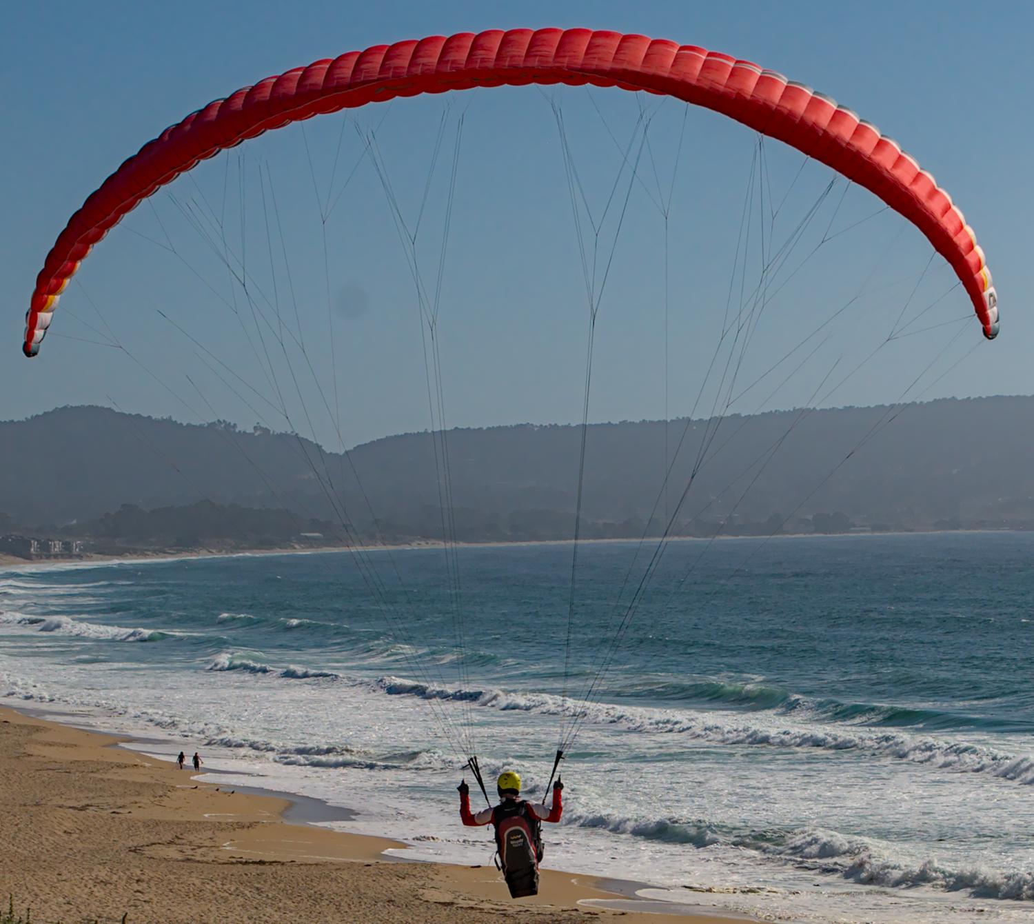
Fig. 8.6 Rear-view of an inflated Hook 3 with symmetric brake deflections

First, the zero-brake values. From this picture the deflection appears to begin near the middle of each semispan. Adding a symmetric margin softens the distribution while keeping the starting point centered at $s=0.5$, so $s_{\text{start},0}=0.3$ and $s_{\text{stop},0}=0.7$ look about right.

The maximum-brake values are more difficult, since they must coordinate with the value of ${\kappa }_b$, but from safety training footage it can be seen that maximum brakes produce a deflection from roughly $s_{\text{start},1}=0.08$ to $s_{\text{stop},1}=1.05$ (where the stopping position exceeds the wing tip to indicate that the wing tip itself experiences a small deflection).

Next, the model needs the maximum distance the brake lines can be pulled. On a real wing the brake lines effectively don’t have a well-defined limit, since a pilot can literally wrap the brake lines around their hand to pull the trailing edge all the way back to the risers, but in practice the airfoil set Fig. 8.4 that defines the deflected profiles is limited to some maximum deflection distance. For that reason, the Suspension lines model uses brake inputs on a scale from 0 to 1, with a maximum brake deflection distance ${\kappa }_b$. The value of ${\kappa }_b$ should maximize the usable range of the brakes without causing the normalized deflection distance ${\overline{\delta }}_d$ (5.1) of any section to exceed the distance supported by the airfoil set. Written as an optimization in terms of (5.14), the goal is to calculate the value of ${\kappa }_b$ such that:

$$\underset{s}{max}\frac{{\delta }_d(s,1,1)}{c(s)}={\overline{\delta }}_{d,\text{max}}$$

Checking the airfoil set used for this model (Fig. 8.4), define ${\overline{\delta }}_{d,\text{max}}=0.203$. Solving the optimization problem determines ${\kappa }_b=0.426[m]$. This procedure is unfortunately convoluted, but in summary: for this specific airfoil set, the foil’s chord distribution, and these brake position parameters, the model can allow the brake lines to be pulled a maximum distance of $42.6[cm]$.

To check the model fit, plot the undeflected and deflected trailing edge to compare with the reference photos:

Fig. 8.7 Niviuk Hook 3 23 brake distribution, ${\delta }_{bl}=0.25$ and ${\delta }_{br}=0.5$

Fig. 8.8 Niviuk Hook 3 23 brake distribution, ${\delta }_{bl}=1.00$ and ${\delta }_{br}=1.0$

8.3.3. Line drag

The third group of parameters (5.26) for the suspension line model determine the aerodynamic drag of the lines. Because the model is focused on providing functionality instead of a detailed (and tedious) layout of every line, it computes the drag by lumping the total area of the lines into a small number of points. For this demonstration, satisfactory results can be achieved with just two points (one for each semispan) and crude estimates of the true line area distribution.

First, the total line length for this wing is listed directly in the technical specs, ${\kappa }_L=218[m]$. Next, ${\kappa }_L$ must be multiplied by the average diameter of the lines ${\kappa }_d$ to get their total surface area. Although a complete set of diameters for each line segment are given in the “Lines Technical Data” section, computing an accurate distribution would require their detailed layout; instead, with lower sections of the cascade averaging $2.8[mm]$ and upper sections using $0.6[mm]$ lines, a good starting point is to assume an average diameter of ${\kappa }_d=1[mm]$. Next, the area is divided into the two control points, which must be positioned at the area centroids of their group of lines. For an approximate model such as this, the positions of the points are easiest to estimate visually; using Fig. 8.6 they appear to be around ${\mathbf{r}}_{CP/R}=⟨-0.5c_{\text{root}},\pm 1.75,1.75⟩$. Lastly, each lumped line area is assigned a drag coefficient; because the lines are essentially cylinders, a suitable drag coefficient is simply $C_{d,l}=1$ [20].

8.4. Payload

The final component model of the paraglider system is for the harness. This component is responsible for positioning the mass of the payload (harness and pilot) as a function of weight-shift, and computing the aerodynamic drag applied to the payload.

The parameters of the model are the total mass of the payload ($m_p$), the vertical distance of the mass centroid below the riser midpoint ($z_{\text{riser}}$), the cross-sectional area of the payload ($S_{\text{payload}}$), the aerodynamic drag coefficient ($C_{d,\text{payload}}$), and the maximum horizontal distance a pilot can displace the centroid using weight-shift control (${\kappa }_w$).

For the total mass, the technical specs list the weight range for the size 23 wing as 65–85 [kg], so $m_p=75\left[\text{kg}\right]$ is a conservative choice.

For the mass centroid, one option is to consider the DHV airworthiness guidelines [48], which specify that the riser attachment points must be “35–65cm above the seat board”, which suggests that $z_{\text{riser}}=0.5\left[\text{m}\right]$ is a reasonable value in most cases. Alternatively, simply look up the technical diagram of a suitable harness; for example, the wing certification flight tests (published in the Hook 3 User Manual, p. 22) list the “harness to risers distance” as 49cm.

For the surface area and its associated drag coefficient, consider [31] (p. 85) or [30] (p. 422); given that 75kg is a lower-than-average payload (so smaller frontal area), and that this is a beginner-grade wing (so a high performance “pod” harness is less likely), a reasonable choice of the area would be $S_{\text{payload}}=0.55\left[{\text{m}}^2\right]$ with an drag coefficient of $C_{d,\text{payload}}=0.8$.

Lastly, when choosing a weight shift limit, underestimates are preferable to overestimates, since an underestimate merely limits the range of behavior the model can produce, whereas an overestimate can produce fictitious behavior; in the absence of a rigorous measurement, a conservative guess is ${\kappa }_w=0.15\left[\text{m}\right]$.